这篇文章主要介绍了Python使用低通滤波器模糊图像,我们介绍了多种不同类型的滤波器核与卷积操作,使用 scipy.ndimage 模块中的滤波器模糊图像,利用 scipy.fftpack 模块的 fft2() 函数实现高斯模糊,介绍了scipy.signal模块的彩色图像频域卷积,需要的朋友可以参考下
使用低通滤波器模糊图像
0. 前言
低通滤波器 (Low Pass Filter, LPF) 过滤了图像中的高频部分,并仅允许低频部分通过。因此,在图像上应用 LPF 会删除图像中的细节/边缘和噪声/离群值,此过程也称为图像模糊(或平滑),图像平滑可以作为复杂图像处理任务的预处理部分。在本节中,我们将学习如何使用不同类型的滤波器核执行图像卷积以模糊图像。
1. 频域中的不同类型的核与卷积
1.1 图像模糊分类
图像模糊通常包含以下类型:
- 边缘模糊 (
Edge) 这种类型的模糊通常通过卷积显式地应用于图像,例如线性滤波器核或高斯核等,使用这些滤波器核可以平滑/去除图像中不必要的细节/噪声。 - 运动模糊 (
Motion) 通常是由于相机在拍摄图像时抖动所产生的,也就是说,摄像机或被拍摄的对象处于移动状态。我们可以使用点扩展函数来模拟这种模糊。 - 失焦模糊 (
de-focus) 当相机拍摄的对象失焦时,会产生这种类型的模糊;我们可以使用模糊 (blur) 核来模拟这种模糊。
接下来,我们创建以上三种不同类型的核,并将它们应用于图像以观察不同类型核处理图像后的结果。
1.2 使用不同核执行图像模糊
(1) 我们首先定义函数 get_gaussian_edge_blur_kernel() 以返回 2D 高斯模糊核用于边缘模糊。该函数接受高斯标准差 ( σ σ σ) 以及创建 2D 核的大小(例如,sz = 15 将创建尺寸为 15x15 的核)作为函数的参数。如下所示,首先创建了一个 1D 高斯核,然后计算两个 1D 高斯核的外积返回 2D 核:
import numpy as np import numpy.fft as fp from skimage.io import imread from skimage.color import rgb2gray import matplotlib.pyplot as plt import cv2 def get_gaussian_edge_blur_kernel(sigma, sz=15): # First create a 1-D Gaussian kernel x = np.linspace(-10, 10, sz) kernel_1d = np.exp(-x**2/sigma**2) kernel_1d /= np.trapz(kernel_1d) # normalize the sum to 1.0 # create a 2-D Gaussian kernel from the 1-D kernel kernel_2d = kernel_1d[:, np.newaxis] * kernel_1d[np.newaxis, :] return kernel_2d
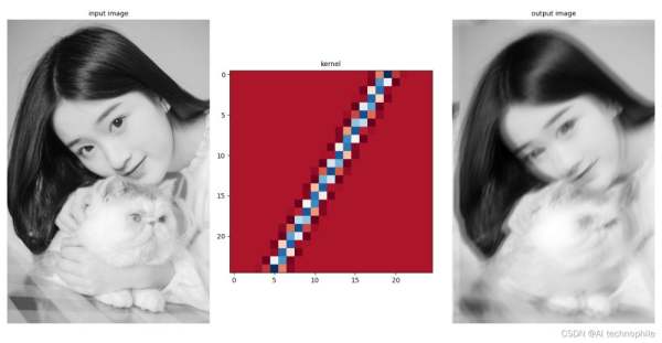
(2) 接下来,定义函数 get_motion_blur_kernel() 以生成运动模糊核,得到给定长度且特定方向(角度)的线作为卷积核,以模拟输入图像的运动模糊效果:
def get_motion_blur_kernel(ln, angle, sz=15): kern = np.ones((1, ln), np.float32) angle = -np.pi*angle/180 c, s = np.cos(angle), np.sin(angle) A = np.float32([[c, -s, 0], [s, c, 0]]) sz2 = sz // 2 A[:,2] = (sz2, sz2) - np.dot(A[:,:2], ((ln-1)*0.5, 0)) kern = cv2.warpAffine(kern, A, (sz, sz), flags=cv2.INTER_CUBIC) return kern
函数 get_motion_blur_kernel() 将模糊的长度和角度以及模糊核的尺寸作为参数,函数使用 OpenCV 的 warpaffine() 函数返回核矩阵(以矩阵中心为中点,使用给定长度和给定角度得到核)。
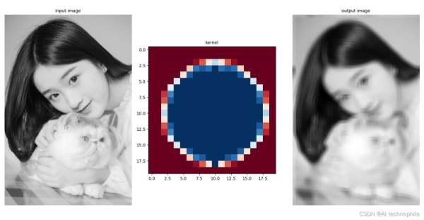
(3) 最后,定义函数 get_out_of_focus_kernel() 以生成失焦核(模拟图像失焦模糊),其根据给定半径创建圆用作卷积核,该函数接受半径 R (Deocus Radius) 和要生成的核大小作为输入参数:
def get_out_of_focus_kernel(r, sz=15): kern = np.zeros((sz, sz), np.uint8) cv2.circle(kern, (sz, sz), r, 255, -1, cv2.LINE_AA, shift=1) kern = np.float32(kern) / 255 return kern
(4) 接下来,实现函数 dft_convolve(),该函数使用图像的逐元素乘法和频域中的卷积核执行频域卷积(基于卷积定理)。该函数还绘制输入图像、核和卷积计算后得到的输出图像:
def dft_convolve(im, kernel): F_im = fp.fft2(im) #F_kernel = fp.fft2(kernel, s=im.shape) F_kernel = fp.fft2(fp.ifftshift(kernel), s=im.shape) F_filtered = F_im * F_kernel im_filtered = fp.ifft2(F_filtered) cmap = 'RdBu' plt.figure(figsize=(20,10)) plt.gray() plt.subplot(131), plt.imshow(im), plt.axis('off'), plt.title('input image', size=10) plt.subplot(132), plt.imshow(kernel, cmap=cmap), plt.title('kernel', size=10) plt.subplot(133), plt.imshow(im_filtered.real), plt.axis('off'), plt.title('output image', size=10) plt.tight_layout() plt.show()(5) 将 get_gaussian_edge_blur_kernel() 核函数应用于图像,并绘制输入,核和输出模糊图像:
im = rgb2gray(imread('3.jpg-600')) kernel = get_gaussian_edge_blur_kernel(25, 25) dft_convolve(im, kernel)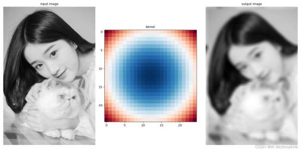
(6) 接下来,将 get_motion_blur_kernel() 函数应用于图像,并绘制输入,核和输出模糊图像:
kernel = get_motion_blur_kernel(30, 60, 25) dft_convolve(im, kernel)
(7) 最后,将 get_out_of_focus_kernel() 函数应用于图像,并绘制输入,核和输出模糊图像:
kernel = get_out_of_focus_kernel(15, 20) dft_convolve(im, kernel)
2. 使用 scipy.ndimage 滤波器模糊图像
scipy.ndimage 模块提供了一系列可以在频域中对图像应用低通滤波器的函数。本节中,我们通过几个示例学习其中一些滤波器的用法。
2.1 使用 fourier_gaussian() 函数
使用 scipy.ndimage 库中的 fourier_gaussian() 函数在频域中使用高斯核执行卷积操作。
(1) 首先,读取输入图像,并将其转换为灰度图像,并通过使用 FFT 获取其频域表示:
import numpy as np import numpy.fft as fp from skimage.io import imread import matplotlib.pyplot as plt from scipy import ndimage im = imread('1.png-600', as_gray=True) freq = fp.fft2(im)(2) 接下来,使用 fourier_gaussian() 函数对图像执行模糊操作,使用两个具有不同标准差的高斯核,绘制输入、输出图像以及功率谱:
fig, axes = plt.subplots(2, 3, figsize=(20,15)) plt.subplots_adjust(0,0,1,0.95,0.05,0.05) plt.gray() # show the filtered result in grayscale axes[0, 0].imshow(im), axes[0, 0].set_title('Original Image', size=10) axes[1, 0].imshow((20*np.log10( 0.1 + fp.fftshift(freq))).real.astype(int)), axes[1, 0].set_title('Original Image Spectrum', size=10) i = 1 for sigma in [3,5]: convolved_freq = ndimage.fourier_gaussian(freq, sigma=sigma) convolved = fp.ifft2(convolved_freq).real # the imaginary part is an artifact axes[0, i].imshow(convolved) axes[0, i].set_title(r'Output with FFT Gaussian Blur, $\sigma$={}'.format(sigma), size=10) axes[1, i].imshow((20*np.log10( 0.1 + fp.fftshift(convolved_freq))).real.astype(int)) axes[1, i].set_title(r'Spectrum with FFT Gaussian Blur, $\sigma$={}'.format(sigma), size=10) i += 1 for a in axes.ravel(): a.axis('off') plt.show()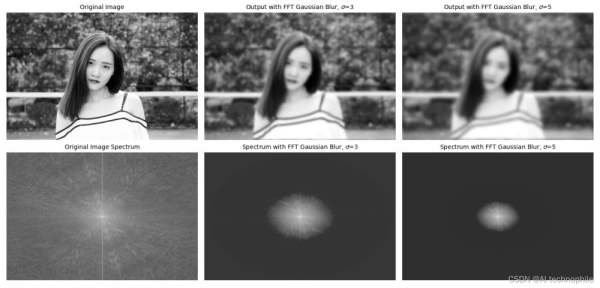
从上图中可以看出,高斯核的标准差 σ σ σ 值越大,输出图像就会越模糊。
2.2 使用 fourier_uniform() 函数
scipy.ndimage 模块的函数 fourier_uniform() 实现了多维均匀傅立叶滤波器。频率阵列与给定尺寸的方形核的傅立叶变换相乘。接下来,我们学习如何使用 LPF (均值滤波器)模糊输入灰度图像。
(1) 首先,读取输入图像并使用 DFT 获取其频域表示:
im = imread('1.png-600', as_gray=True) freq = fp.fft2(im)(2) 然后,使用函数 fourier_uniform() 应用 10x10 方形核(由功率谱上的参数指定),以获取平滑输出:
freq_uniform = ndimage.fourier_uniform(freq, size=10)
(3) 绘制原始输入图像和模糊后的图像:
fig, (axes1, axes2) = plt.subplots(1, 2, figsize=(20,10)) plt.gray() # show the result in grayscale im1 = fp.ifft2(freq_uniform) axes1.imshow(im), axes1.axis('off') axes1.set_title('Original Image', size=10) axes2.imshow(im1.real) # the imaginary part is an artifact axes2.axis('off') axes2.set_title('Blurred Image with Fourier Uniform', size=10) plt.tight_layout() plt.show()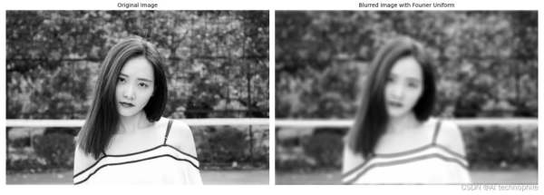
(4) 最后,绘制显示方形核的功率谱:
plt.figure(figsize=(10,10)) plt.imshow( (20*np.log10( 0.1 + fp.fftshift(freq_uniform))).real.astype(int)) plt.title('Frequency Spectrum with fourier uniform', size=10) plt.show()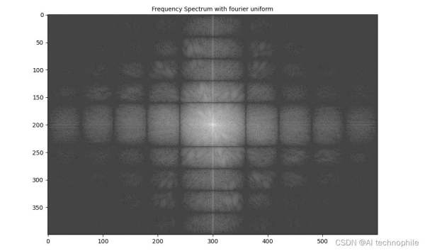
2.3 使用 fourier_ellipsoid() 函数
与上一小节类似,通过将方形核修改为椭圆形核,我们可以使用椭圆形核生成模糊的输出图像。
(1) 类似的,我们首先在图像的功率谱上应用函数 fourier_ellipsoid(),并使用 IDFT 在空间域中获得模糊后的输出图像:
freq_ellipsoid = ndimage.fourier_ellipsoid(freq, size=10) im1 = fp.ifft2(freq_ellipsoid)
(2) 接下来,绘制原始输入图像和模糊后的图像:
fig, (axes1, axes2) = plt.subplots(1, 2, figsize=(20,10)) axes1.imshow(im), axes1.axis('off') axes1.set_title('Original Image', size=10) axes2.imshow(im1.real) # the imaginary part is an artifact axes2.axis('off') axes2.set_title('Blurred Image with Fourier Ellipsoid', size=10) plt.tight_layout() plt.show()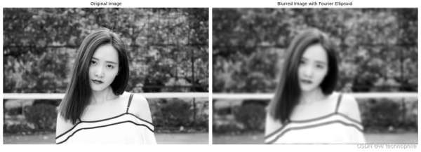
(3) 最后,显示应用椭圆形核后图像的频谱:
plt.figure(figsize=(10,10)) plt.imshow( (20*np.log10( 0.1 + fp.fftshift(freq_ellipsoid))).real.astype(int)) plt.title('Frequency Spectrum with Fourier ellipsoid', size=10) plt.show()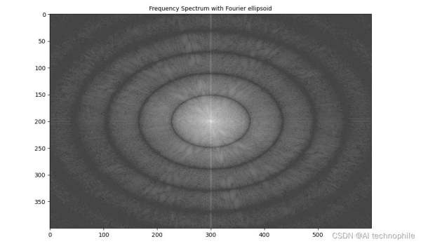
3. 使用 scipy.fftpack 实现高斯模糊
我们已经学习了如何在实际应用中使用 numpy.fft 模块的 2D-FFT。在本节中,我们将介绍 scipy.fftpack 模块的 fft2() 函数用于实现高斯模糊。
(1) 使用灰度图像作为输入,并使用 FFT 从图像中创建 2D 频率响应数组:
import numpy as np import numpy.fft as fp from skimage.color import rgb2gray from skimage.io import imread import matplotlib.pyplot as plt from scipy import signal from matplotlib.ticker import LinearLocator, FormatStrFormatter im = rgb2gray(imread('1.png-600')) freq = fp.fft2(im)(2) 通过计算两个 1D 高斯核的外积,在空间域中创建高斯 2D 核用作 LPF:
kernel = np.outer(signal.gaussian(im.shape[0], 1), signal.gaussian(im.shape[1], 1))
(3) 使用 DFT 获得高斯核的频率响应:
freq_kernel = fp.fft2(fp.ifftshift(kernel))
(4) 使用卷积定理通过逐元素乘法在频域中将 LPF 与输入图像卷积:
convolved = freq*freq_kernel # by the Convolution theorem
(5) 使用 IFFT 获得输出图像,需要注意的是,要正确显示输出图像,需要缩放输出图像:
im_blur = fp.ifft2(convolved).real im_blur = 255 * im_blur / np.max(im_blur)
(6) 绘制图像、高斯核和在频域中卷积后获得图像的功率谱,可以使用 matplotlib.colormap 绘制色,以了解不同坐标下的频率响应值:
plt.figure(figsize=(20,20)) plt.subplot(221), plt.imshow(kernel, cmap='coolwarm'), plt.colorbar() plt.title('Gaussian Blur Kernel', size=10) plt.subplot(222) plt.imshow( (20*np.log10( 0.01 + fp.fftshift(freq_kernel))).real.astype(int), cmap='inferno') plt.colorbar() plt.title('Gaussian Blur Kernel (Freq. Spec.)', size=10) plt.subplot(223), plt.imshow(im, cmap='gray'), plt.axis('off'), plt.title('Input Image', size=10) plt.subplot(224), plt.imshow(im_blur, cmap='gray'), plt.axis('off'), plt.title('Output Blurred Image', size=10) plt.tight_layout() plt.show()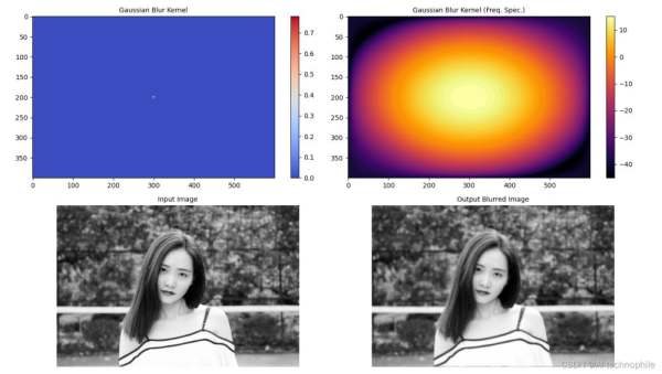
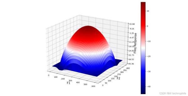
(7) 要绘制输入/输出图像和 3D 核的功率谱,我们定义函数 plot_3d(),使用 mpl_toolkits.mplot3d 模块的 plot_surface() 函数获取 3D 功率谱图,给定相应的 Y 和Z值作为 2D 阵列传递:
def plot_3d(X, Y, Z, cmap=plt.cm.seismic): fig = plt.figure(figsize=(20,20)) ax = fig.gca(projection='3d') # Plot the surface. surf = ax.plot_surface(X, Y, Z, cmap=cmap, linewidth=5, antialiased=False) #ax.plot_wireframe(X, Y, Z, rstride=10, cstride=10) #ax.set_zscale("log", nonposx='clip') #ax.zaxis.set_scale('log') ax.zaxis.set_major_locator(LinearLocator(10)) ax.zaxis.set_major_formatter(FormatStrFormatter('%.02f')) ax.set_xlabel('F1', size=15) ax.set_ylabel('F2', size=15) ax.set_zlabel('Freq Response', size=15) #ax.set_zlim((-40,10)) # Add a color bar which maps values to colors. fig.colorbar(surf) #, shrink=0.15, aspect=10) #plt.title('Frequency Response of the Gaussian Kernel') plt.show() (8) 在 3D 空间中绘制高斯核的频率响应,并使用 plot_3d() 函数:
Y = np.arange(freq.shape[0]) #-freq.shape[0]//2,freq.shape[0]-freq.shape[0]//2) X = np.arange(freq.shape[1]) #-freq.shape[1]//2,freq.shape[1]-freq.shape[1]//2) X, Y = np.meshgrid(X, Y) Z = (20*np.log10( 0.01 + fp.fftshift(freq_kernel))).real plot_3d(X,Y,Z)
下图显示了 3D 空间中高斯 LPF 核的功率谱:
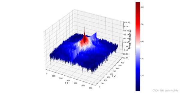
(9) 绘制 3D 空间中输入图像的功率谱:
Z = (20*np.log10( 0.01 + fp.fftshift(freq))).real plot_3d(X,Y,Z)
(10) 最后,绘制输出图像的功率谱(通过将高斯核与输入图像卷积获得):
Z = (20*np.log10( 0.01 + fp.fftshift(convolved))).real plot_3d(X,Y,Z)
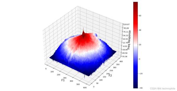
从输出图像的频率响应中可以看出,高频组件被衰减,从而导致细节的平滑/丢失,并导致输出图像模糊。
4. 彩色图像频域卷积
在本节中,我们将学习使用 scipy.signal 模块的 fftconvolve() 函数,用于与 RGB 彩色输入图像进行频域卷积,从而生成 RGB 彩色模糊输出图像:
scipy.signal.fftconvolve(in1, in2, mode='full', axes=None)
函数使用 FFT 卷积两个 n 维数组 in1 和 in2,并由 mode 参数确定输出大小。卷积模式 mode 具有以下类型:
- 输出是输入的完全离散线性卷积,默认情况下使用此种卷积模式
- 输出仅由那些不依赖零填充的元素组成,
in1或in2的尺寸必须相同 - 输出的大小与
in1相同,并以输出为中心
4.1 基于 scipy.signal 模块的彩色图像频域卷积
接下来,我们实现高斯低通滤波器并使用 Laplacian 高通滤波器执行相应操作。
(1) 首先,导入所需的包,并读取输入 RGB 图像:
from skimage import img_as_float from scipy import signal import numpy as np import matplotlib.pyplot as plt im = img_as_float(plt.imread('1.png-600'))(2) 实现函数 get_gaussian_edge_kernel(),并根据此函数创建一个尺寸为 15x15 的高斯核:
def get_gaussian_edge_blur_kernel(sigma, sz=15): # First create a 1-D Gaussian kernel x = np.linspace(-10, 10, sz) kernel_1d = np.exp(-x**2/sigma**2) kernel_1d /= np.trapz(kernel_1d) # normalize the sum to 1.0 # create a 2-D Gaussian kernel from the 1-D kernel kernel_2d = kernel_1d[:, np.newaxis] * kernel_1d[np.newaxis, :] return kernel_2d kernel = get_gaussian_edge_blur_kernel(sigma=10, sz=15)
(3) 然后,使用 np.newaxis 将核尺寸重塑为 15x15x1,并使用 same 模式调用函数 signal.fftconvolve():
im1 = signal.fftconvolve(im, kernel[:, :, np.newaxis], mode='same') im1 = im1 / np.max(im1)
在以上代码中使用的 mode='same',可以强制输出形状与输入阵列形状相同,以避免边框效应。
(4) 接下来,使用 laplacian HPF 内核,并使用相同函数执行频域卷积。需要注意的是,我们可能需要缩放/裁剪输出图像以使输出值保持像素的浮点值范围 [0,1] 内:
kernel = np.array([[0,-1,0],[-1,4,-1],[0,-1,0]]) im2 = signal.fftconvolve(im, kernel[:, :, np.newaxis], mode='same') im2 = im2 / np.max(im2) im2 = np.clip(im2, 0, 1)
(5) 最后,绘制输入图像和使用卷积创建的输出图像。
plt.figure(figsize=(20,10)) plt.subplot(131), plt.imshow(im), plt.axis('off'), plt.title('original image', size=10) plt.subplot(132), plt.imshow(im1), plt.axis('off'), plt.title('output with Gaussian LPF', size=10) plt.subplot(133), plt.imshow(im2), plt.axis('off'), plt.title('output with Laplacian HPF', size=10) plt.tight_layout() plt.show()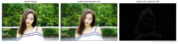
如上图所示,高斯 LPF 可以用于模糊图像,而拉普拉斯 HPF 则可以用于提取图像中的细节/边缘(这些部分对应于图像中的高频分量)。
小结
在图像上应用低通滤波器会删除图像中的细节/边缘和噪声/离群值,称为图像模糊(或平滑),图像平滑可以作为复杂图像处理任务的预处理部分。在本节中,我们介绍了多种不同类型的滤波器核与卷积操作,使用 scipy.ndimage 模块中的滤波器模糊图像,利用 scipy.fftpack 模块的 fft2() 函数实现高斯模糊,还介绍了基于 scipy.signal 模块的彩色图像频域卷积。
到此这篇关于Python使用低通滤波器模糊图像的文章就介绍到这了,更多相关Python低通滤波器模糊图像内容请搜索0133技术站以前的文章或继续浏览下面的相关文章希望大家以后多多支持0133技术站!
以上就是Python使用低通滤波器模糊图像功能实现的详细内容,更多请关注0133技术站其它相关文章!


